Basic tutorial

In this notebook we exemplify how to analyze an image-based dataset using troutpy. We will identify unsegmented transcripts and characterize them using diverse functions.

0. Dataset for the tutorial

In this tutorial we will use a Xenium mouse brain dataset that has been pre-formated for troutpy’s usage. See “Formatting spatialdata for troutpy” tutorial to first format your dataset. The dataset can be downloaded from this Zenodo record

1. Import packages

import spatialdata as sd
import troutpy as tp
import scanpy as sc

2. Load SpatialData object

We first load the SpatialData dataset (see info at section 0) using the SpatialData read_zarr function

sdata = sd.read_zarr("./data.zarr")  # please modify the path to your conveniece
sdata

SpatialData object, with associated Zarr store: /media/sergio/Meninges/troutpy/rois/xenium_msbrain_5k/data.zarr
├── Images
│     └── 'morphology_focus': DataTree[cyx] (5, 9300, 8049), (5, 4650, 4025), (5, 2325, 2012), (5, 1162, 1006), (5, 581, 502)
├── Labels
│     ├── 'cell_labels': DataTree[yx] (9300, 8049), (4650, 4025), (2325, 2012), (1162, 1006), (581, 502)
│     └── 'nucleus_labels': DataTree[yx] (9300, 8049), (4650, 4025), (2325, 2012), (1162, 1006), (581, 502)
├── Points
│     └── 'transcripts': DataFrame with shape: (<Delayed>, 15) (3D points)
├── Shapes
│     ├── 'cell_boundaries': GeoDataFrame shape: (9289, 1) (2D shapes)
│     ├── 'cell_circles': GeoDataFrame shape: (9191, 2) (2D shapes)
│     └── 'nucleus_boundaries': GeoDataFrame shape: (9249, 1) (2D shapes)
└── Tables
      └── 'table': AnnData (9191, 5006)
with coordinate systems:
    ▸ 'global', with elements:
        morphology_focus (Images), cell_labels (Labels), nucleus_labels (Labels), transcripts (Points), cell_boundaries (Shapes), cell_circles (Shapes), nucleus_boundaries (Shapes)

3. Processing cellular information & cell type definition

In case cell types haven’t been identified from segmented cells, we will identify them. In this case, we simply filter low quality cells, normalize its gene expression and perform leiden clustering, prior to manual annotation of cell types. In case your dataset already contains annoated cell types, this step can be skipped

adata = sdata["table"]
adata.raw = adata.copy()

all_cells = adata.shape[0]
sc.pp.filter_cells(adata, min_genes=10)
sc.pp.filter_cells(adata, min_counts=30)
sc.pp.filter_genes(adata, min_cells=3)

print(f"Proportion of cells retained after filtering: {adata.shape[0] / all_cells:.2%}")

Proportion of cells retained after filtering: 99.93%

We next perform normalization and log-transformation.

adata.layers["raw"] = adata.X.copy()
sc.pp.normalize_total(adata)
sc.pp.log1p(adata)

We then cluster cells to identify populations

sc.tl.pca(adata)
sc.pp.neighbors(adata, n_neighbors=10)
sc.tl.umap(adata)
sc.tl.leiden(adata, key_added="leiden", resolution=0.6)

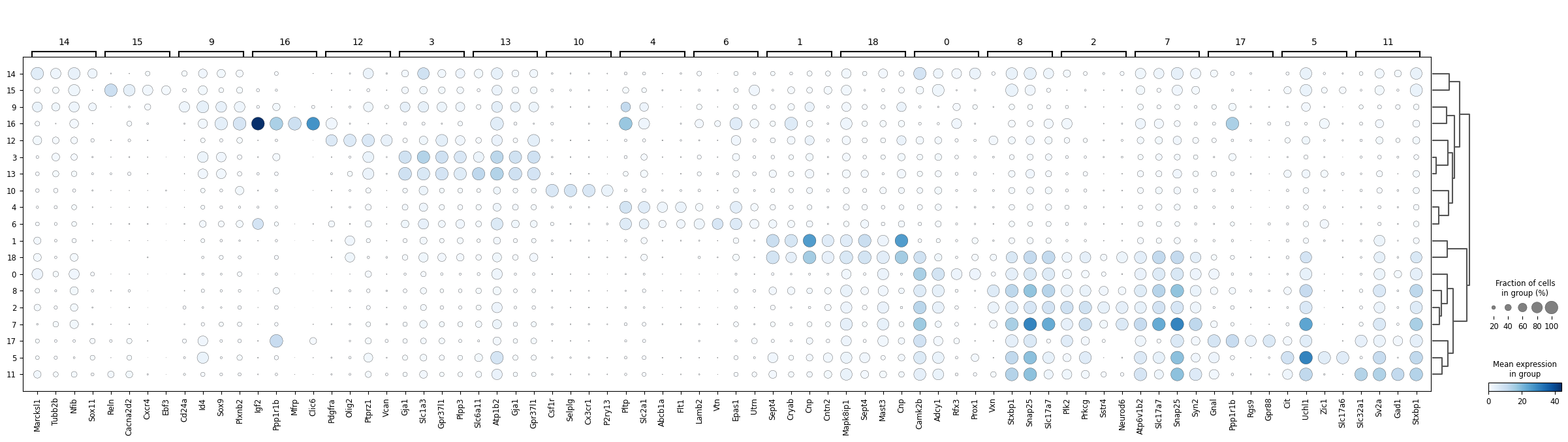
sc.tl.rank_genes_groups(adata, groupby="leiden")
sc.tl.dendrogram(adata, groupby="leiden")
sc.pl.rank_genes_groups_dotplot(adata, groupby="leiden", n_genes=4, cmap="Blues")

WARNING: Default of the method has been changed to 't-test' from 't-test_overestim_var'
WARNING: It seems you use rank_genes_groups on the raw count data. Please logarithmize your data before calling rank_genes_groups.

dict_anno = {
    0: "DG",
    1: "Oligodendrocytes",
    2: "CA1-2",
    3: "Astrocytes",
    4: "Endothelial",
    5: "EXC neurons Thal.",
    6: "SMC/Pericytes",
    7: "CA3",
    8: "EXC. neurons CTX",
    9: "Ependymal cells",
    10: "Microglia",
    11: "INH neurons",
    12: "OPC",
    13: "Astrocytes",
    14: "SGZ Neuroblasts",
    15: "Cajal-Retzius",
    16: "Choroid plexus",
    17: "INH neurons CP",
    18: "Oligodendrocytes",
}
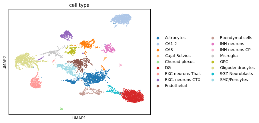
adata.obs["cell type"] = adata.obs["leiden"].astype(int).map(dict_anno)
sc.pl.umap(adata, color="cell type", palette="tab20")
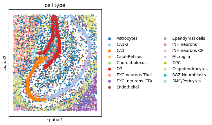
sc.pl.spatial(adata, spot_size=30, color="cell type", palette="tab20")

4. Segmentation-free analysis

We use troutpy.tl.segmentation_free_sainsc to perform segmentation-free analysis, using a Sainsc (Müller-Bötticher et.al 2024). Essentially, for each transcript in the tissue, we bin it into pixels of the specified binsize, in ums. We also filter background signal based on the background_filter parameter. Since spatial datasets are typically sparse, especially at those resolutions, we also apply gaussian blurring of the signal, adjusted by gaussian_kernel_key parameter.

After binning, filtering and smoothing each pixel, we compute a cosine similarity between each pixel’s signature and the cell-type signatures defined. In our case, we define cell type signatures using the mean expression of the cell types, defined by a column in sdata['table'].obs. Column name can be specified using ```celltype_key``.

For each bin/pixel, we obtain a cosine similarity to each cell type. For our purposes, we will just retain the maximum cosine similarity per pixel to any cell type and which cell type is that value originating from. This will be then added to the per-transcript information as new columns in sdata['transcripts']

tp.pp.segmentation_free_sainsc(sdata, binsize=5, celltype_key="leiden", background_filter=0.2, gaussian_kernel_key=2.0)

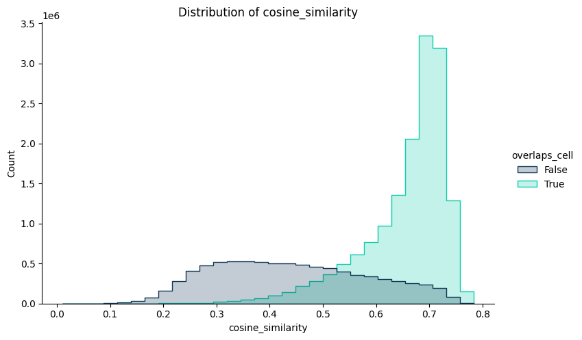
Since we included in the analysis all transcripts, we can then compare the cosine similarity of the transcripts segmented to cells and those who were not. This will allow us to classify unassigned RNA in two groups:

• RNA that locallyresembles segmented cells (cell-like)

• RNA that have a local composition different from segmented cells(other uRNA)

# 3) Histogram of scores
tp.pl.histogram(sdata, x="cosine_similarity", hue="overlaps_cell", palette="troutpy")

Next, we will use the output of segmentation and segmentation-free analysis to non-cell-like transcripts. For this, we will employ the command troutpy.pp.define_urna. Essentially, extracellular transcripts will be defined as those:

• Located outside segmented cells

• Have a cosine similarity to cell type signatures below the threshold set by percentile_threshold, which is computed using only cellular pixels.

# 4) Define extracellular
tp.pp.define_urna(sdata, layer="transcripts", method="sainsc", percentile_threshold=5)

Cosine similarity threshold for extracellular definition: 0.48941171169281006

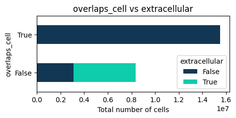
We can visualize how many transcripts considered as non-cell like (here-extracellular), among the ones that were not origially segmented

# 5) Crosstab / pie / heatmap
tp.pl.crosstab(sdata, yvar="extracellular", xvar="overlaps_cell", normalize=False, cmap="troutpy", kind="barh", stacked=True, figsize=(5, 2))

<Figure size 500x200 with 0 Axes>

5. Gene-centric exploration of uRNA compopsition

5.1 Exploring uRNA abundance and proportion

After defining which unassigned RNA does not come from missegmentation, we focus on characterizing the remaining uRNA . First, we will quantify how abundant is each uRNA type (each gene) in the uRNA pool, comparing it to noise levels. We implemented troutpy.tl.quantify_overexpression to identify overexpressed genes relative to a noise threshold.

Essentially, this function computes a threshold based on the counts of specified control features and compares gene counts against this threshold to determine overexpression. The function calculates log-fold changes for each gene, annotates metadata with these results. It returns updated spatial data along with per-gene scores and the calculated threshold

control_codewords = ["negative_control_probe", "unassigned_codeword", "deprecated_codeword", "genomic_control_probe", "negative_control_codeword"]

tp.tl.quantify_overexpression(
    sdata, layer="transcripts", codeword_key="codeword_category", control_codewords=control_codewords, gene_key="gene", percentile_threshold=99.5
)

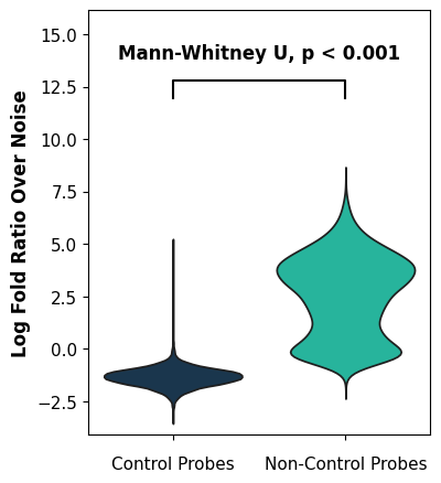
We visualize how many genes are present in the uRNA pool over noise levels. As you can see, all control probes are below noise levels (as expected) and some non-control genes are found in the uRNA pool over noise levels

tp.pl.logfoldratio_over_noise(sdata, test_method="auto")

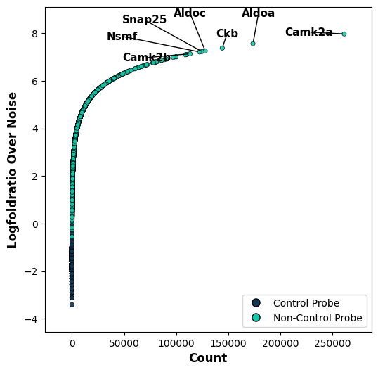
We want to explore which genes are the most enriched ones over noise levels. For this, we visualize a scatter plot with each point representing a single gene. We visualize the uRNA counts in comparison with the logFoldRatio over noise. We identify that specific genes have a high abundance in the uRNA pool.

tp.pl.metric_scatter(sdata, x="count", y="logfoldratio_over_noise", label_top_n_x=7, label_top_n_y=5, label_bottom_n_x=0, label_bottom_n_y=0, size=20)

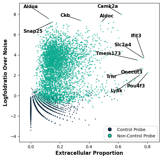
Despite knowing it’s contribution to the uRNA pool can be important information, it could simply be that a gene that is highly expressed intracellularly is also highly abundant outside cells due to diverse reasons. Therefore, to complement the uRNA abundance information it will be useful to know also, for each gene, which proportion of its detected RNA is kept unassigned. For this we use the function tp.tl.extracellular_enrichment. This will highlight genes that tend to be more detected outside segmented cells.

tp.tl.extracellular_enrichment(sdata)

We can now visualize both metrics, the uRNA abundance, and the uRNA proportion, side by side across genes. We observe that different genes present different patterns:

• Genes with low uRNA/extracellular proportion (i.e. Aldoa)- are simply highly abundant genes

• Genes with high uRNA proportion but low uRNA abundance- suggest expression patterns in uRNA that is not well captured by segmentation

• Genes with both high uRNA abundance and proportion represent highly expressed genes that are very enriched outside segmented cells. Represent clear patterns

tp.pl.metric_scatter(
    sdata,
    x="extracellular_proportion",
    y="logfoldratio_over_noise",
    label_top_n_x=7,
    label_top_n_y=5,
    label_bottom_n_x=0,
    label_bottom_n_y=0,
    size=5,
    linewidth=0.1,
)

5.2 Exploring spatial variability and uRNA patterning

We can also explore other patterns such as the spatial variability of individual uRNA genes. For this, we will first bin the uRNA transcripts into bins, same as we did for segmenation-free analysis. We adjust the square_size parameter to vary the size of squares. Then we will compute moranI.

tp.pp.aggregate_urna(sdata, gene_key="gene", square_size=50)
tp.tl.spatial_variability(sdata, gene_key="gene", n_neighbors=10)

We can then identify the most spatially variable genes in the uRNA spectrum. All gene-specific uRNA-related information, including uRNA abundance, proportion, spatial variability etc. is stored in sdata['xrna_metadata'].var. We can find the most variable genes, with a higher moranI using:

sdata["xrna_metadata"].var.sort_values(by="moran_I", ascending=False).head(5)

	count	logfoldratio_over_noise	control_probe	p_value_Poisson	intracellular_proportion	extracellular_proportion	logfoldratio_extracellular	moran_I	moran_pval_norm	moran_var_norm	moran_pval_norm_fdr_bh
Camk2a	261445	7.970620	False	0.0	0.377494	0.622506	-1.762111	0.742294	0.0	0.000022	0.0
Adcy1	86277	6.861959	False	0.0	0.521692	0.478308	-1.175092	0.675149	0.0	0.000022	0.0
Map2	109117	7.096817	False	0.0	0.464694	0.535306	-1.403373	0.622938	0.0	0.000022	0.0
Sptbn2	56148	6.432387	False	0.0	0.403648	0.596352	-1.652203	0.613253	0.0	0.000022	0.0
Kif5a	71066	6.668005	False	0.0	0.431416	0.568584	-1.537990	0.613056	0.0	0.000022	0.0

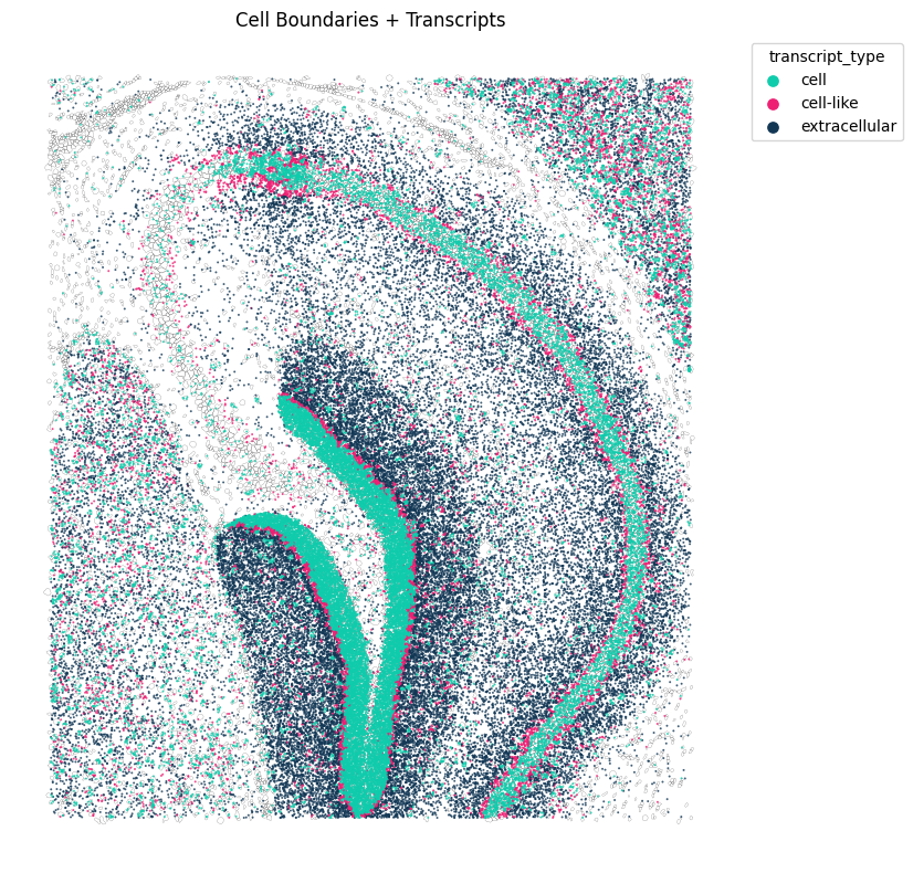
Next we can the distribution of of some of these genes in the space using troutpy.pp.spatial_transcripts. In this case, Adcy1

tp.pl.spatial_transcripts(sdata, gene_list=["Adcy1"], scatter_size=2, boundary_linewidth=0.1)

No transformation matrix found. Proceeding without transformation.

(<Figure size 800x800 with 1 Axes>,
 <Axes: title={'center': 'Cell Boundaries + Transcripts'}>)

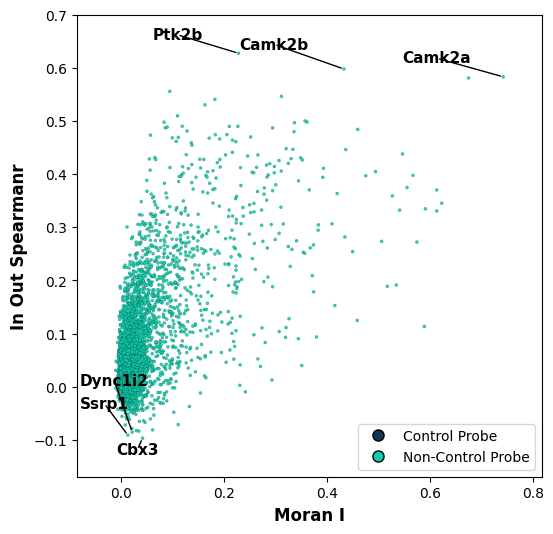
One important part when understanding uRNA is identifying patterns that differ from those found in segmented cell. For this, we can test for intra-extracellular correlation (extracellular here means uRNA). A requirement for this function is to pre-compute extracellular bins using tp.pp.aggregate_urna

sdata["transcripts"]["gene"] = sdata["transcripts"]["gene"].astype("category")
tp.pp.aggregate_urna(sdata, gene_key="gene", square_size=50)
tp.tl.in_out_correlation(sdata, n_neighbors=20)

tp.pl.metric_scatter(
    sdata, x="moran_I", y="in_out_spearmanR", label_top_n_x=0, label_top_n_y=3, label_bottom_n_x=0, label_bottom_n_y=3, size=5, linewidth=0.1
)

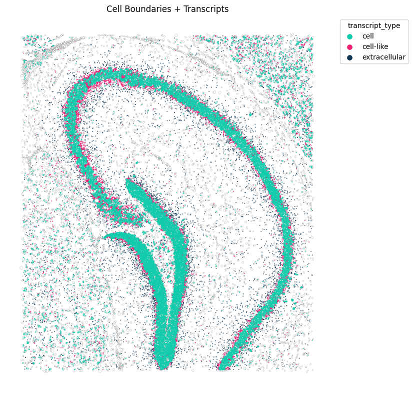
We can visualize how expression in and out cells compare, fr one of the genes with highest spearman’s intracellular-extracellular correlation

tp.pl.spatial_transcripts(sdata, gene_list=["Ptk2b"], scatter_size=2, boundary_linewidth=0.1)

No transformation matrix found. Proceeding without transformation.

(<Figure size 800x800 with 1 Axes>,
 <Axes: title={'center': 'Cell Boundaries + Transcripts'}>)

5.3 Filtering uRNA genes

For some analysis, we might want to only keep part of the genes, the ones showing relevant characteristics. For instance, we might want to only keep genes clearly found above noise and that are not control probes. This we can do with:

tp.pp.filter_urna(sdata, min_logfoldratio_over_noise=7, gene_key="gene")  # filter out genes with a logfoldratio over noise below 7.
tp.pp.filter_urna(sdata, gene_key="gene", control_probe=True)  # filter control probes

sdata["xrna_metadata"].var.shape

(11, 13)

6. Identifying uRNAs source

For the selected genes, we identify each uRNA’s source. For this, we compute a source score, which represents the probability of a cell being the origin of each uRNA. We will use the function tp.tl.compute_source_score to identify the source cell types that may contribute to the extracellular RNA detected in spatial transcriptomics data.

tp.tl.compute_source_score(sdata, layer="transcripts", gene_key="gene", lambda_decay=0.1, celltype_key="cell type", n_jobs=1)

The resulting source score is stored in sdata['source_score'], in AnnData format, where .X represents the source score for each transcript (obs) across cell types (var). Furthermore, other information such as the ID of the closest cell expressing the transcript, distance to the closest cell expressing the transcript and closest celltype are also stored.

sdata["source_score"]

AnnData object with n_obs × n_vars = 519413 × 17
    obs: 'gene', 'distance', 'closest_cell', 'closest_celltype'
    obsm: 'spatial'

6.1 Assesing diffusion

We can use the source score information for several purposes. First, we can assess wether, for each gene, the distances in relation to their closest potential source cells follows a rayleigh distribution, which would suggest diffusion as an origin of the pattern.

tp.tl.assess_diffusion(sdata, gene_key="gene", distance_key="distance")

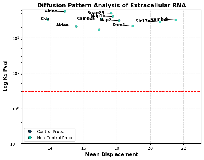
We can visualize the output of our diffusion test. We show the -Log p-value of a the kolmogorov smirnov test done between the distribution of distances fitted to rayleigh distribution and the measured ones. Red line indicates significance, with everything above the red line representing a distribution of distances different from rayleigh (diffusion) distribution. Y axis represents the mean distance at which the uRNA are located from their potential source

As observed, in this example all genes exhibit distributions that do not match diffusion patterns

tp.pl.diffusion_results(sdata, label_top_n_y=10, y_logscale=True)

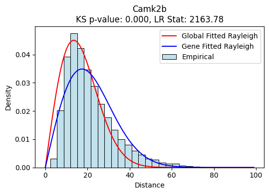
We can also visualize the distributions and the fited raileigh curves for each gene. We find a gene-specific one fitted distribution, which is fitted only with the counts of the gene of interest, as well as a global one, fitted with all genes. Gene-fitted distributions are used for KS testing. As seen in these example, we observe a clear enrichment of uRNAs at higher distances in comparison with expected (40-60), which results in a very low p-value

tp.pl.gene_distribution_from_source(sdata, ["Camk2b"])

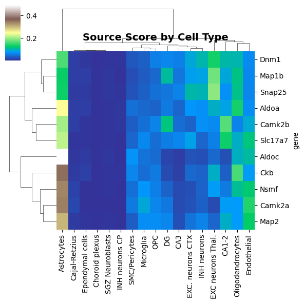
We can also visualize, for each gene, their potential uRNAs source based on cell type expression and physical proximity

tp.pl.source_score_by_celltype(sdata, figsize=(6, 6), cmap="terrain")

6.2. Cell-specific uRNAs source score

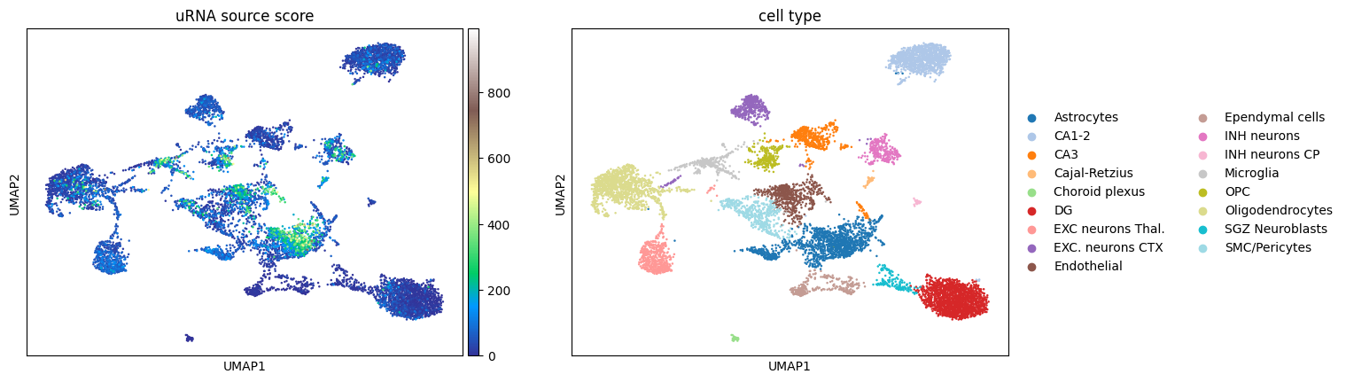
From our source score analysis, performed previously, we also obtain a per-cell uRNA source score, stored in sdata['table'].obs as a column called urna_source_score This score represents, for each cell, how many uRNAs from the uRNA pool cn be attributed to each cell. We can simply visualize the scores for each cell

sc.pl.umap(sdata["table"], color=["urna_source_score", "cell type"], cmap="terrain", title="uRNA source score", vmax="p99.995")

WARNING: The title list is shorter than the number of panels. Using 'color' value instead for some plots.

7 Target scores and cell-cell contacts inferred from uRNA

We also want to compute target score

tp.tl.compute_target_score(sdata, layer="transcripts", lambda_decay=0.1, copy=False, celltype_key="cell type", gene_key="gene")

We want to use this information to compute enhanced cell-cell contact. The idea is that non-technical uRNA must represents RNA from protrusions and, thus, it can be used as a proxy of cell-cell contact.

tp.tl.cell_contacts_with_urna_sources(sdata, spatial_key="spatial", cell_type_key="cell type", distance=20)

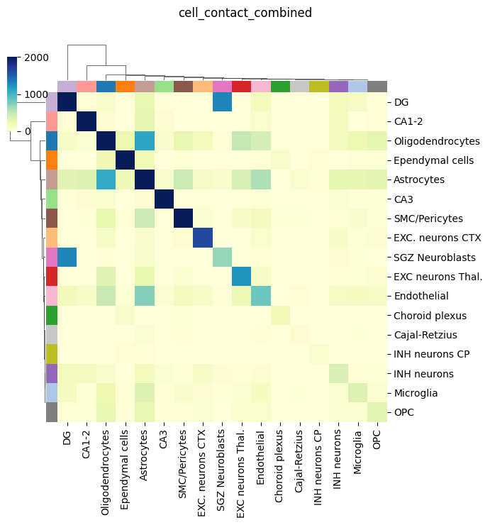
We can visualize the combined cell-cell contacts between paired cell types. This includes both proximity between cell bodies and uRNA-mediate cell-cell contacts

tp.pl.cell_type_contacts(sdata, celltype_key="cell type", figsize=(7, 7), dendrogram_ratio=0.1, cmap="YlGnBu", key="cell_contact_combined", vmax=2000)

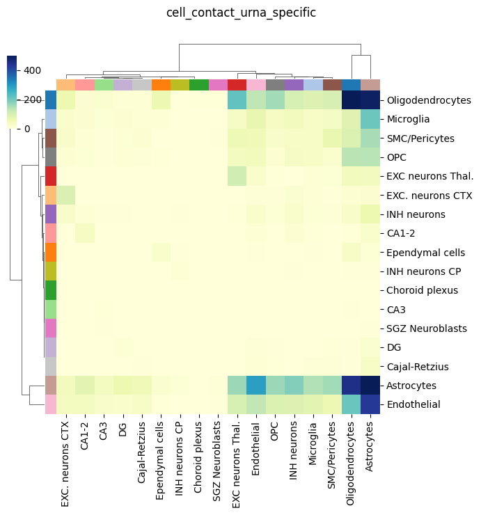
We can finally also visualze only the cell-cell contacts inferred from uRNA. As observed, they are not that many as the cell-body ones, but they are clearly enriched for some cell types, including Endothelial, oligodendorcytes and astrocytes. These cell types are known to present abundant but short protrusion, which are expected to be captured by this appriach. Furthermoe, these metric is clearly assimetrical, since cell proximity is only considered for a target cell (receiver, columns) if a certain uRNA with a defined source (sender,rows) is found in its vicinity

tp.pl.cell_type_contacts(
    sdata, celltype_key="cell type", figsize=(7, 7), dendrogram_ratio=0.1, cmap="YlGnBu", key="cell_contact_urna_specific", vmax=500
)

We will finally save the final object for our internal use

sdata.write("./data_filt.zarr")  # please modify the path to your conveniece